tl;dr
Behavioral testing for time series forecasting models can be used to assess their adaptability to sudden changes in historical data. In this blog post, I am using the Prophet framework to evaluate the model’s response to permanent shocks within a time series.
What is behavior testing?
Behavior testing is a methodology for evaluating the adaptability of a model to sudden changes in historical data. It is a form of stress testing that simulates shocks within the time series and observes the model’s response. This approach can be used to assess the model’s ability to adapt to new patterns and eventually stabilize.
Why is behavior testing important?
Time series forecasting models are often trained on historical data and used to predict future trends. However, these models may not be able to adapt to sudden changes in the data, such as economic downturns or shifts in consumer behavior. Behavior testing can be used to evaluate the model’s ability to handle such changes and provide insights into its adaptability.
Lets dive into it
Example data
I will use a dataset from the M4 competition to demonstrate the behavior testing approach. The dataset contains 100,000 time series from different domains and various frequencies. For the demonstration purposes, I randomly picked a monthly time series from the dataset - the time series with the ID M54.
Generating a permanent shock
The first step is to introduce a simulated permanent shock within the time series. This shock can mimic sudden changes, such as economic downturns, shifts in consumer behavior, or anomalies affecting the data. In this example, I will simulate a positive permanent shock by multiplying the time series values by a factor of 1.2. I use the forecasting horizon of 12 months to evaluate the model’s prediction performance.
At t = 12 the shock is introduced. In the illustration below, the simulated values are shown in orange. Green is the last observation in the training data.
The prediction performance is evaluated for 12 time steps after the shock was introduced (t = 12, t = 13, …, t = 23). In this example I will use the mean absolute percentage error (MAPE) as the evaluation metric.
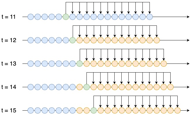
To get a robust approximation of the adaptibility of the model, I will repeat the experiment 10 times. Each time I will randomly pick a new date to introduce the shock. The following plot shows the 10 randomly selected intervention dates, where the shock is introduced.
The plots are created using the plotly library. You can zoom in and interact with the graphs.
The global results
In the table below the global results are shown. Later in this blog post, I will deep dive into a single simulation run in more detail. The results are aggregated across all simulations. The median adaption time in this example is 1 month, while the mean adaption time is 4.5 months with a standard deviation of 5.32 months.
What is the adaption time?
The adaption time is the number of months required for the model to regain a level of accuracy comparable to its pre-shock performance.
| Statistic | Value |
|---|---|
| Runs | 10.000 |
| Median | 1.000 |
| Mean | 4.500 |
| Std | 5.315 |
| Min | 0.000 |
| Max | 12.000 |
The distribution of the adaption time is shown in the histogram below. The majority of the simulations (6 out of 10) required less than 2 months to recover from the shock. However, in 3 cases the model did not recover at all in the evaluation period of 12 months.
The following table shows the aggregated results for each simulation run. One simulation run consists of 12 evaluation steps before the shock, in order to establish a benchmark prediciton performance, and 12 evaluation steps after the shock.
sim_mape is the mean absolute percentage error (MAPE) of the Prophet model on the simulated data.
sim_mape_std is the standard deviation of the MAPE across the 12 simulated time steps.
benchmark_mape is the MAPE of the Prophet model on 12 months before the simulation shock.
adaption_time is the number of months required for the model to regain a level of accuracy comparable to its pre-shock performance.
| run | sim_mape | sim_mape_std | benchmark_mape | adaption_time |
|---|---|---|---|---|
| 0 | 0.165 | 0.091 | 1.067 | 0 |
| 1 | 0.219 | 0.053 | 0.194 | 7 |
| 2 | 0.144 | 0.010 | 0.049 | 12 |
| 3 | 0.300 | 0.198 | 1.319 | 0 |
| 4 | 0.189 | 0.008 | 0.039 | 12 |
| 5 | 0.238 | 0.129 | 0.333 | 2 |
| 6 | 0.213 | 0.030 | 0.189 | 0 |
| 7 | 0.354 | 0.134 | 0.582 | 0 |
| 8 | 0.548 | 0.208 | 0.291 | 0 |
| 9 | 0.110 | 0.021 | 0.060 | 12 |
What does simulation run 1 look like?
In this section, I will deep dive into a single simulation run, run 1. The plot below shows each evaluation step of the simulation run. The blue line is the actual time series, the green line is the simulated time series, and the red line is the Prophet model’s prediction with a prediction horizon of 12 months.
The shock is introduced at evaluation step 12. The prior 12 evaluation steps are used to establish a benchmark prediction performance. The MAPEs before and after the shock are shown in the next plot.
This plot shows the MAPEs before and after the shock, blue and red line correspondingly. The prediction performance before the shock is 0.194 (grey horizontal line). It is used to assess how long it takes for the model to recover from the shock.
As expected the MAPE jumps significantly after the introduction of the shock. The model needs 7 months to recover from the shock and regain a level of accuracy comparable to its pre-shock performance.
Conclusion
Behavior testing can be used to evaluate the adaptability of a time series forecasting model to sudden changes in historical data. In this blog post, I used Prophet, one of the most widely used time series forecasting frameworks. I am not advocating for Prophet, but I am using it as an example to demonstrate the behavior testing approach.
The results show that the model needs on average 4.5 months to recover from the shock and regain a level of accuracy comparable to its pre-shock performance. This finding is true to this specific time series in combination with the Prophet model. The results will vary for other time series and models.
Hopefully, this blog post provides you with a new perspective on time series forecasting models and their evaluation. If you are interested in behavioral testing for time series forecasting models, I have created a python package called flair. The package is still in its early stages, but I am working on adding more features and improving the documentation.
If you have any questions or feedback, please reach out to me on Twitter.